Colors and Borders in Microsoft Excel What are they, what are they for and how to use them to improve the aesthetics of your documents?

Users who wish to manage a spreadsheet to perfection they will need to know all the secrets that the tool has to add borders and colors.

Which will make the work be done in less time and the results, to expose the information, be consistent with a professional style. Also, this will allow to generate different types of layout to Excel documents.

In order for you to become an expert and prepare spreadsheets perfectly, you will have to read the following paragraphs. We will show you the steps you will need to do to modify borders and colors to cells, rows, columns and graphs.

What elements of a spreadsheet can I add borders and colors to in Excel?

One of the reasons borders should be used in a spreadsheet is because it gives a unique look to tables and any other illustrations used to display information.

This is because borders of different colors can be added to cells, letters, columns, rows, and charts.. There are a large number of designs that can be chosen, which allow you to change not only the color of the lines, but also their thickness and number.

Border styles What are all that I can add in my spreadsheet?

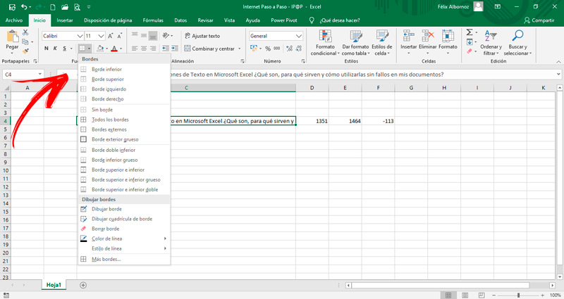
You must bear in mind that the styles that we will show you are taken as a reference from the selection cell that you have chosen. The types of borders you can add to a spreadsheet are as follows:

• Lower: It is one of the most used and that is why it is in the first place. It is useful when you want to set column titles, you can also use it when you want to display the total of a column at the end of the data.
• Higher: You can also use it in the same way as the previous one, but in the opposite situation. Both borders have a fine line that provides a clean style to the tables and information that are displayed.
• Left: This type of border is used when you want to detail and separate horizontal concepts in a table or in the preparation of forms.
• Law: It corresponds to the same situation as the leading edge, but it can be used in situations in which the design of the box or table ends.
• All edges: When you have a table with many columns and rows and the information that exists can make the reader dizzy, it is necessary to use this type of border. With this tool you will limit all the cells that exist in the selection.
• External edges: if you have information in a box and you want to highlight it only on the outside, you will have to use this layout. It is the opposite style to the previous border since it does not mark the internal cells, it only makes lines in the selection limit.
• Thick outer: It fulfills the same function as the previous border but the line used for this design is thick.
• Lower Double: In case you need to highlight a selection with a double line at the bottom, you will have to use this type of layout.
• thick bottom: If what you need is to place a line that has a thickness much greater than the common one to place it at the end of the selection, you will have to use this type of border.
• Upper and lower: there are tables that do not need to be demarcated on their left and right sides, so this type of border is very useful when there are cases in which you want to give an elegant style so that the user can have a good reading.
• Thick top and bottom: It has the same functions as the leading edge, but in this case the bottom line is double the width.
• Double top and bottom: The same thing happens as in the last 2 designs with this type of border, but in this format both lines are thick.

Learn step by step how to modify the colors of your spreadsheets

By default, Microsoft Excel displays lines that exist at the intersection of columns and rows. Therefore, the style it has is transparent in color, but if you want to modify this you can do it with very simple steps.

Pay attention to the following guides:

In letters

To change the colors of the letters you must follow these steps:

• Select the cells you want to change.
• Right click on the selection and choose the option “Format the cells…”.
• Go to the tab “Font”.
• Look for the option “Color”.
• Click on the arrow to display the color palette. When you have chosen the one you like the most, you will have to select “To accept”.

in cells

In case you want to modify the colors of the cells, do the following:

• With the mouse select the cell, or the set of them, that you want to modify.
• Go to the Home tab and look for the group of functions “Font”.
• Choose “Fill color”.
• When you click on the drop-down menu you will have to choose the tone that you like the most from the color palette.

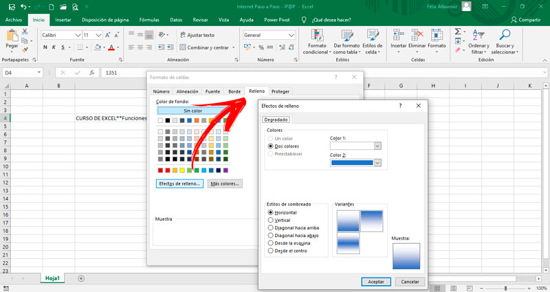
In case you don’t want to have a complete fill color and you need to give it a different style you should follow these steps:

• Once you have selected the cells you want to edit, right click on them.
• Look for the option “Cell format…” and click on the tab “Filling”.
• Then tap on “Fill effects…”.
• You will have to choose if you want a color or the colors, so you will have to select them by displaying the arrow at the end of the fields “Colour 1:” Y “Color 2:”.
• Then you will need to choose the shading style. This means whether you want to do it horizontally, vertically, or another way.

In Charts

When you have graphics and want to change their color, you will have to do this step by step:

• Click on it. You will see that the angles turned into white dots.
• Then right click and select the tool “Filling”which will appear independently next to the illustration.
• Choose the one you need from the range of colors. You can also give it a gradient effect, choosing the option that bears that name.

If you prefer, you can change the filling for an image that you can choose from your computer or from the Internet. For this, you will have to choose the option “Image”after you have clicked on “Filling”.

Steps to insert borders to your spreadsheets and make them more dynamic

The steps that we will show you below can be done with any type of border. Let’s see what you need to do:

• Choose the cell, rows or columns to which you want to add a border.
• Click on the tab “Start”.
• In the group “Font” you will have the tool “Edge” represented by a box.
• Click on the arrow to open the menu.
• Choose the border style that suits you best.

In case you have a table with different types of borders and you want to add some, but if you use the defaults If you modify the direction of the form, you will have the option to draw the border manually.

For this you will have to choose the function “draw borders” and in this way you can drag the mouse through the places where they need to incorporate lines. you can also draw grids quickly by simply passing the mouse over the different sectors. You must bear in mind that this function will remain activated until you click on it again.

If for some reason you make a mistake and want to erase an edge, you will have to use the tool “Clear border”. As is the case with the “draw borders”this function will remain active until you click on it again.