How to make a pivot table in Microsoft Excel? step by step guide

Microsoft Excel allows you to work with different tables in a single board. This generates that the user can have a dynamism with which you can consult different data by clicking on the filters you have created.

These tools are known as pivot tables. and they are widely used in spreadsheets due to the efficiency and speed with which they are created. But they have some secrets that you should know.

So that you can become a professional in the handling of pivot tableswe will show you below all the tips you should know to create the best query box.

When is it more convenient to use a pivot table than a normal one?

A dynamic table offers the possibility of being able to change the columns and rows to show a certain order.. In this way, it will be possible to filter more comfortably, since only the searched data will be displayed.

Instead, a normal table will always show filtering by columns or rows, making the information could not be stated in an easier way to understand different parameters.

Steps to create a pivot table in an Excel spreadsheet

The steps you will have to do to create a pivot table are:

• Go to the cell in which you want the pivot table to be.
• Click on the tab “Insert”.
• Then choose in the group “Boards” the tool “Dynamic table”.
• Choose the data you want to analyze by activating the option “Select a table or range” and placing the selection in the field “Table or range:”.
• Find where you want the table report to appear. It can be in a new or existing spreadsheet.
• When you’re done, you’ll need to click “To accept”.
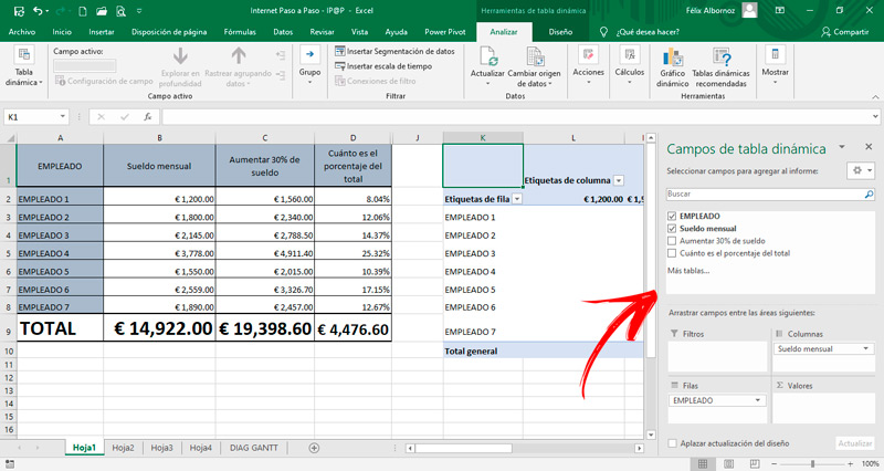
• Then you will see that the table has been inserted in the place you have set. What you have to do now is to include the rows and columns so that the table is according to your needs.