How to alphabetize the data in your spreadsheets with Microsoft Excel filters? step by step guide

One of the most used functions in Microsoft Excel is sort and filter. This is due to the advantages that it presents so that the user can find the information quicklytaking into account certain criteria.

Although it is not a difficult tool to handle, you have to be careful. If misused, it could distort formulas and thus generate incorrect information.

In order for you to become an expert in Excel, we will show you the steps you must do so that you can use this function in a professional way.. Don’t miss any paragraph.

Sort and filter tool When is it convenient to use it and what are the advantages of doing it?

The sort and filter tool is very useful when you take into account some considerations. For example, if it is known that each time the filter is pressed, the data will change order, so many times the information may be poorly related in relation to the other data.

Also, If this function is used incorrectly, only one column can be sorted, leaving the rest of the sheet unchanged.. This will imply that the data will end up out of order and the information will not be correct.

If these points are taken into account and the tool is handled with care, the sort and filter function is very convenient to use, even more so when you have an average knowledge of Microsoft Excel.

Steps to automatically alphabetize data from your spreadsheets

So you can sort, alphabetically, the data you have in your spreadsheet you will have to do the steps that we will show you below:

ranks

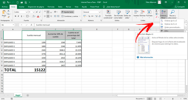
Click on the header of the data range you want to filter, then follow these directions:

• In the Home tab look for the group “Edition”.
• Choose the function “Sort and filter”.
• Next, click on “Filter”.
• You will see that in the place where you placed the cursor, the content of the cell appears with an arrow on the right side. If you see that it takes the data that you want to reorder it, you must create a cell above the place where you chose. This will make it miss the first number you have with the arrow right now.
• When you press the drop-down menu, the option you you can filter from smallest to largest or largest to smallest. Click on any of the 2 and you will see how the entire column was relocated in an orderly manner.

Boards

The steps that you will have to carry out to order a table are the same that we explained to you with a range. The difference that exists is that the cell you will choose will be combined.

In this case, when you order from highest to lowest or vice versa, the system will take as the default order the last column of the set of the combined cell that appears under the title.

Learn step by step how to master the tool in Excel documents

Next, We will show you all the secrets you need to know so you can successfully master the tool in Excel documents:

Numbers

To filter by numbers it is necessary that the column contains numerical data and not another type of format. If you want to perform this task you must follow this process:

• Select the range you want to order.
• Then go to “Edition” and click on “Sort and Filter”.
• Click on “Filter”.
• Go back to the data you have and click on the filter arrow.
• When the window is displayed you will have to select the tool “Filters by number”. And then set the condition so that Microsoft Excel returns the related values.

With this tool you can filter under criteria that are related to “Equal to…”, “Greater or equal to…” , “Among…”, “Top 10 best…”, “Above average” or perform a custom filter, among other conditions.

dates and times

In case you have data related to dates and times, you can sort them by following this step by step:

• Choose the range you want to filter.
• Click on “Edition”Then in “Sort and Filter” and lastly in “Filter”.
• Now, you are going to have to press the filter arrow and choose the option “Date Filters”.

You can choose filters “Is equal to…”, “Among…”, “Before…” Y “After…” in which an additional window will open in which you must choose the conditionals so that Excel can return the values ​​that have those characteristics.

In addition, you can choose tools that are “Next week”, “Last month”, “This year” or choose a “Custom Filter”among many other tools.

You can do the same steps for formats with hours.

Multiple columns or rows

When you want to sort multiple columns or rows, you will have to select the entire box, apply filter and then choose the option “Custom order…”.

Next, you will need to follow this guide:

• Once the pop-up opens you will be able to choose by column or sort by cell values.
• You can also do it, if you have different colors, for this feature.
• Then, you will have to choose if you want the order to be left to right or top to bottom.
• Once you have chosen these criteria you can choose so that you can see the results from highest to lowest or vice versa.

Cell, font, or icon colors

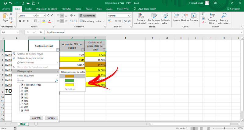
The criteria that we will show you below are the same for these 3 themes, but you must keep in mind that it will only work if you have different colors, fonts or icons in the cells.

The process you must follow is as follows:

• When you have done the filtering, you will have to click on the arrow to display a pop-up window.
• Look for the option “Filter by color” (You will also find fonts or icons, depending on what you need).
• The last thing left for you to do is choose the color of the cells to perform the filtering you need.

custom list

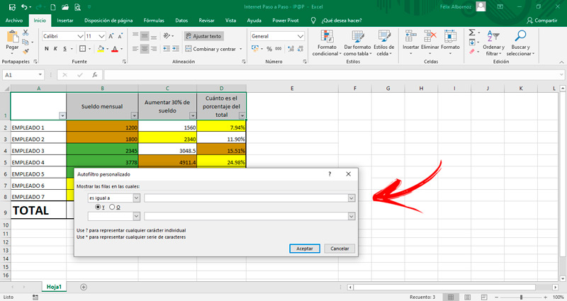
In the personalized list you will have the possibility to work with different formats that you have in the range of data that you want to order. In this way, you will be able to choose when you click on the option “Organize” and filter tool “Custom order…”.

With this you will be able to access different options that will allow you to manage the values ​​of a column, order according to the cells and add or delete levels. In addition, you will be able to establish if the data contains headers or not.

Differentiating uppercase from lowercase

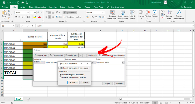
In order to access this type of filtering, you will have to follow the steps to access the personalized list, then you will have to click on “Options…” and check the box “Sensitive uppercase from lowercase”.

From left to right

To the As with case sensitivity, you can also filter from left to right. For this, you will have to access “Custom order…”then click on “Options…” and enable the option “Sort left to right”.

This will make all your data have a horizontal priority and not a vertical order.

By partial values ​​in a column

Once you are in the tool “Custom order…” you will have to locate the option “Column” and then click on the tool “Sort by”.

When you click on the arrow you will find a list with all your data, you only need to choose one of these so that Microsoft Excel can order them with this criterion.

Ranges within a larger range

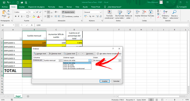
Excel allows you to order values ​​within a larger range. This means that the first thing the program will do is establish a certain order of a range and then it will order again within it by another condition.

To perform this “underfiltered” you will have to access the custom order and then choose the tool “Sort by”. Next, you will have to click on the arrow to choose “Cell Values”colors (if applicable) or format icons, according to the nature of the information you want to order.