How to do simple mathematical operations in a Microsoft Excel spreadsheet? step by step guide

One of the most frequent uses of Excel is to choose this program to perform mathematical operations. Therefore, it will be necessary for you to know in detail how to do each of the operations.

For it, We have prepared this post. We will show you all the steps you must take to be able to add, subtract, multiply and divide a range of numbers. You can do this easily and quickly.

But this is not the only thing we will see, We will also teach you statistical functions so you can get the average and the maximum and minimum values ​​of a group of numbers.. Let’s get started!

What to keep in mind before performing mathematical operations in Microsoft Excel?

Microsoft Excel is characterized by being a simple program in terms of the indications that the user must carry out. Although it is true that this is an advantage, many times it also becomes a drawback if the formulas are not known to be displayed correctly.

Every time you want to perform some mathematical operation, you must take into account that you will have two options to include the data table. You can do it by entering the formulas manually, or by selecting them with the mouse.

If you are going to do it by using the mouse, you will have to choose all the data you want to add, subtract or whatever you need and then select the function within the ribbon.

On the other hand, if you are going to do it manually because you already have some practice in handling formulas, You should keep in mind that all formulas must be preceded by the equals sign (=).

In addition, each time you choose the data range you will have to open parentheses, write the first cell in which the information is found, enter the semicolon (;)set what the last cell is, and then close the parentheses.

From this it follows that, if you have data with negative signs, the system will take it as such, so you must bear in mind that if you do not want to have this variation in the result, you will have to eliminate these factors.

Also, when you perform mathematical operations you can make the mistake of making a circular reference. For example, if you are adding 3 cells and the result of one of them depends on the sum you want to perform, you will have this type of error. Which is represented by a blue line with two circles at its ends.

To solve these problems you will have to correct all the references that are related and depending on each other.

Steps to perform arithmetic math operations in an Excel spreadsheet

The steps that you will have to carry out to do mathematical operations in a Microsoft Excel spreadsheet are the following:

Add

To add you will have to follow these steps:

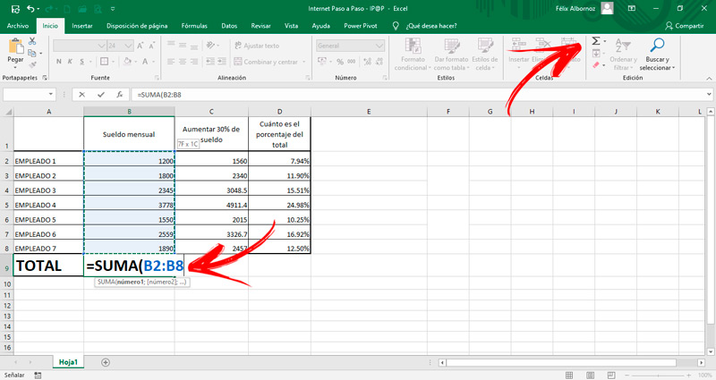
• Select the data you want to add. To do this, press the left mouse button and move it through all the amounts.
• Then go to the tab “Formulas” search in the group “Function Library” the function “Autosum”.

You can also do it by choosing the function “Mathematics and trigonometrics”. For this you will have to place the cursor in the place where you want the formula to return the result. Then, when you have a window open, you will have to select the data you want to add and then choose “To accept”.

There is a much easier way and that is by typing “=SUM(”then press the key “Shift” and with the arrow keys select all the data. When you’re done press 2 times “Enter”.

Subtract

When you want to perform a subtraction you should know that Microsoft Excel does not have a subtraction function, but it does have an addition function for negative numbers.. So you will have to perform the same steps that we show you for that function, but you will have to add the negative sign to the data that you want to be subtracted.

Split

If what you are looking for is to divide two numbers, you must do these steps:

• Place the cursor in the cell in which you want to obtain the result.
• go to “Formulas”
• Choose “Mathematics and trigonometrics”.
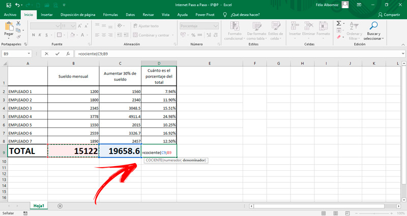
• Look for the formula “QUOTIENT”.
• The numerator and denominator and then tap on “Enter”.

You can also do it manually:

• Write the equal sign in the corresponding cell.
• Then introduce the word quotient.
• Next, without leaving any spaces, press the Open Parenthesis key.
• With the directional arrows choose the numerator.
• Click on “Enter”.
• Select the denominator.
• To finish press twice on “Enter”.

Multiply

To multiply you will have to do the following:

• Choose the place where you need the result to appear.
• Click on the menu “Formulas”.
• Click on the tool “Mathematics and trigonometrics”.
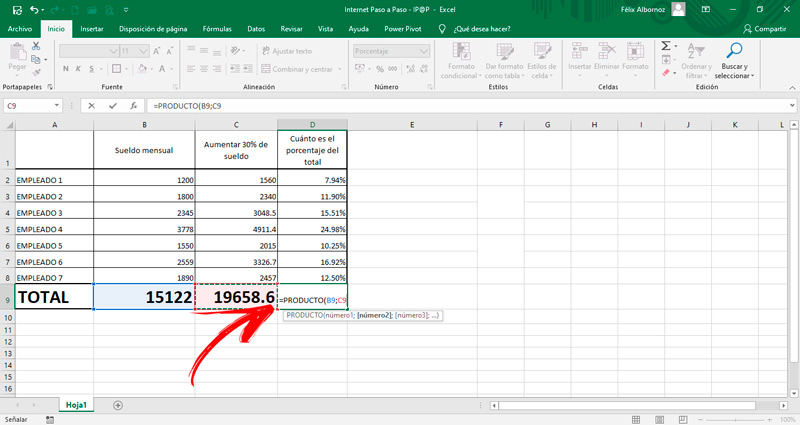
• Choose “PRODUCT”.
• Choose each number and then click on the key “Enter”.

If you prefer, you can perform this task without using the mouse:

• Write in the cell that should return the product the sign “=” either “+”.
• Then select a term using the arrow keys.
• Without leaving space press “*”.
• This way you choose all the products you need. When finished, click on “Enter”.

learn how perform simple statistical operations in Microsoft Excel

When you need to perform basic statistical operations, you must take into account the steps that we will indicate below:

Calculate Average

To calculate the average of a group of numbers, you will have to place the cursor in a cell that you want to return the result to and then follow this guide:

• On the menu “Formulas” select the tool “More Features”.
• Look for the option “Statistics” and choose the function “AVERAGE”.
• Next, a window will open in which you will have to click on the arrow to choose the data group from which you want to obtain the average.
• To finish press the key “Enter”.

There are some jobs where you just need to get the average information, but you don’t want to incorporate it into your data sheet. For these cases, you must select all the data and see at the bottom of the screen. You will find 3 automatic data that Microsoft Excel offers you, one of them is the average.

Calculate Percentage

You should keep in mind that the percentage is a ratio or a division between two numbers. In order to find this relationship you will have to do the following guide:

• In “Formulas” click on “Mathematics and trigonometrics” and choose the tool “QUOTIENT”.
• Select the numbers you want to compare.
• You will see a result in so much by one. If you want to show it as a percentage you will have to select this number and then right click and choose the tool “Cell format…”.
• Choose the tab “Number” and in “Category” look for the option “Percentage”.

This will make the result appear to you as a percentage.

Set Minimum and Maximum

To set the minimum number you will have to:

• Choose where you want the minimum value of a data range to appear.
• go to “More Features” and choose “Statistics”.
• Find the tool “MIN”.
• A window will open in which you will have to select all the data in which you want to find the minimum value.
• Click on “Enter”

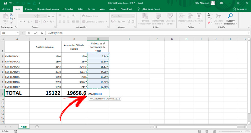
In the same way that you used to get a minimum value, you can also set maximum values. The only thing that will change in the steps that we have shown you is that you will have to choose the function “MAX” instead of “MIN”.