How to perform an interpolation in a Microsoft Excel spreadsheet? step by step guide

Index:

UPDATED ✅ Do you want to know how to interpolate data or ranges in Excel like an expert? ⭐ ENTER HERE ⭐ and Learn all about it

The degree of scope that Excel hasto study known relationships and work with functions, it is very wide. Therefore, many people do not know all the power that this calculation tool.

A somewhat complicated task is to estimate values based on known intervals. That is, establish as precisely as possiblewhich is the number taking certain values as reference.

Due to this there is the data interpolation technique, which we will talk about in the following paragraphs. We will teach you the steps you will take to estimate values quickly and safely. Don’t miss out on anything.

What is a data interpolation and what is it used for in my spreadsheet?

data interpolation It is a mathematical tool used to estimate data are within a known range. By knowing the extreme values, it is possible to interpret the ones that exist within that set. The opposite of interpolation is known as extrapolation and are the data found out of range known.

There are different methods to know the internal points. So the results will be rough estimates which will vary according to the type of method. Among the best known are linear interpolation, quadratic or parabolic and polynomial.

These methods are useful in practice for estimate values from known data. For example, one can estimate the number of tourists who visited Barcelona in 2019 based on specific data obtained in 2017.

Therefore, can be applied to any type of information. Whether the environmental temperature in a certain area of our country or Europe, the housing density, students enrolled in an educational establishment and up to amount of years of average life discriminated by gender of people.

This means that Microsoft Excel is an excellent tool to use it and obtain estimates by means of the data interpolation.

Types of interpolation What are all the ones that exist and can be done in Excel?

The types of interpolation that you can use in Excel to estimate values within a known set are the following:

Linear

Among the different types of interpolation that exist, the easiest method is the linear one.. This is because the possible solutions of the variable X it is only one. Also, joining two points on a graphwe can now draw the line, so find the pairs X₀; Y Y X₁; Y₁it has fewer steps.

This does not mean that this method not be effective nor is it much better than the otherssince it is not possible to determine exactly which one is better if the behavior of the curve is not taken into account.

For this function the formula is used:

Y+{[(X-X)]/(X₁-X)]}*(Y₁-Y).

You can also know the equation of the line by means of the following function:

AXIS(known_y;known_x) for determine the constant a.
EARRING(known_y;known_x) for set the slopethat is b.

parabolic

The parabolic function or also known as quadratic or level 2 polynomialpresents a graph with a minimum or maximum and has the equation formula y=a+bx+cx2. The function is a polynomial which is used to estimate values is y= a + b(xx) + c(xx)(xx₁).

To work in Excel you can substitute the values of the equationor use formulas like COINCIDE and INDEX.

Level 3 Polynomial

function is used y = anxn + … + a1x + ao ; with n=3. In this way it can be determined that a is a0, a1, a2, a3 Y x is x0, x1, x2, x3.

To use Excel and set the vector to you must create this formula:

=ESTIMATE.LINEAR(y;x^(1;2;3;4))

Level 4 Polynomial

Same as him level 3 polynomial can be executed “quantity n” of polynomials, so the treatment is the same from level 3 up to number n.

In this way we can conclude that the method of degree 4 has the same steps and identical features to solve for a value within a known interval as degree 3.

Steps to interpolate data or ranges in a Microsoft Excel spreadsheet

You can then find the steps what you must do to interpolate data within a known range using Microsoft Excel. We will show you a guide for a linear function, a parabolic function and for polynomials of level 3 and 4.

Let’s see them:

Linear

To use a linear interpolation in excel You will have to divide the task into two stages.

The first thing you will have to do are these steps:

Go to the tab “Formula” and then look in the menu “Function Library” the tool “Search and reference”.
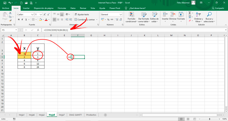
When you click on it will open a windowyou will have to choose the function “COINCIDE”. Since this way you will find a relative position inside the matrix.
choose as lookup value a cell in which you want to get the data.
Then select matrix From the axis X.
In match type you will have to choose number 1since if you choose 0 it will be exact or if you choose number -1 you will have higher value result.

The value you will get is equal to 1. This means that between Y values match the estimate you’re looking for.

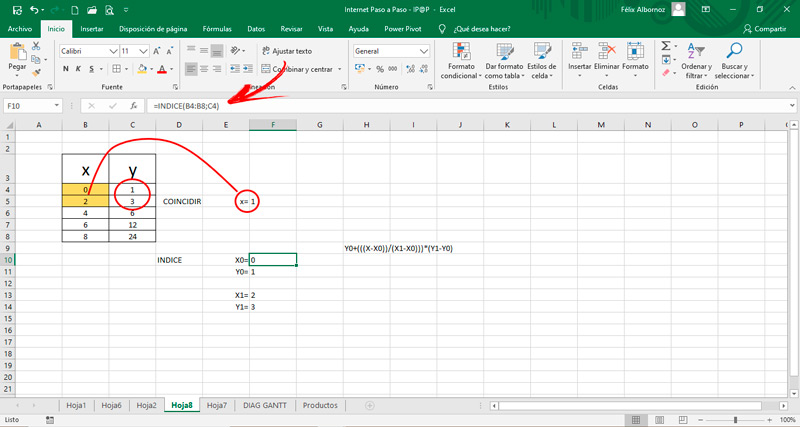
Now you must use the INDEX formula to set the values X;Y and X₁;Y₁.

To do this, follow these steps:

Use the formula INDEX(array; value of Y when it is the first term).
This way you can get the values you are looking for.
When you already have the four values you will have to replace in the formula Y+(((XX))/(X₁-X)))*(Y₁-Y).
You will get the value of Y. That means it’s the estimated value when X is between 2 values.

parabolic

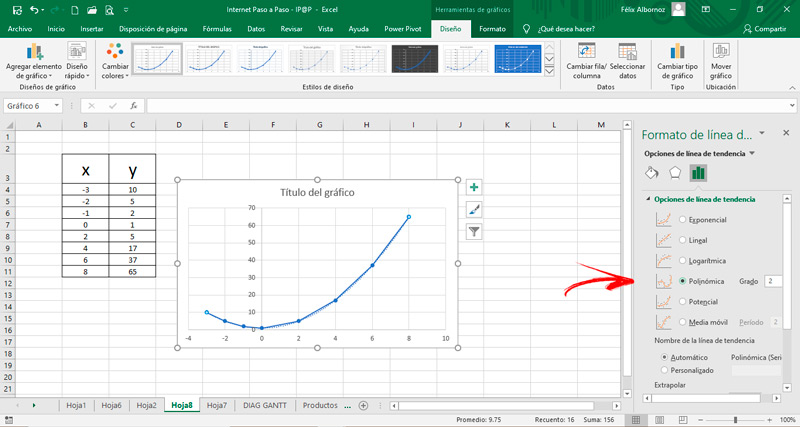
Looking up the equation type y=a+bx+cx2 we’ll do it for graphic medium To find the parabolic method. You can also do it as we took it with the function COINCIDE and INDEXbut we want to show you an easier method for simple cases.

The steps to follow are those:

once you have entered the values of X and of Y select the matrix.
go to “Insert” and then click on “Recommended Graphics”.
Look for the option “Dispersion (XY)” and click on it.
Choose the graphic that suits you best.
Right click on the line that was drawn.
Click on the option “Add trend line…”.
Choose the function “polynomial” and then write “two” in the countryside “Degree:”.
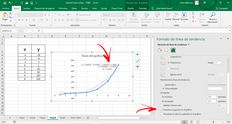
Scroll down and check the boxes “Spot Intersection”, “Display equation on graph” Y “Display R-squared value on chart”. This will allow you to get all data what do you need to find the values you want from Y.

Level 3 Polynomial

The steps that you will have to do are the same that we show you for the parabolic function. once you have all data loaded in a truth table insert a drawing and then set the trend line.

To finish you must check the same boxes and you will get the formula you need to get any value of Y.