Microsoft Excel Statistical Functions What are they, what are they for and how can I apply them to my spreadsheets without errors?

When working with these types of programs users have the opportunity to have a large number of functions that allow them to process data, information and numbers in a much easier and more practical way, without the need to have advanced knowledge on the subject.

This is how functions allow you to process a large number of data and get answers quickly. But it is no secret to anyone that there are many functions available in the Microsoft programso it is very difficult to know them all.

According to this and knowing the importance of each of these elements, here we are going to explain a little more how they work and how you can apply them in your spreadsheetfor this, follow in detail everything that we will teach you in the post.

What is a statistical function in Excel and what is it used for in my documents?

Excel Statistical Functions allow you to calculate all the mathematical operations that are related to the analysis of data stored in a spreadsheet. All this helps to get the data entry number or the average value of the data.

In this way it can be said that statistics is a mathematical discipline which enables study the different ways of summarizing, collecting and drawing conclusions from a series of data under study. This is how this function microsoft allows to make a statistical analysis of informationwhere it is necessary to have formulas to obtain the values ​​of the mean, mean variance, standard deviationamong many others.

Some of the functions most used by users of this program are the “Average, count, MAX, MIN, mode, frequency” among many others that are available there. In addition, it should be mentioned that these tools are available practically in all the versions of excelI know so much for free or paid versions.

List of all Excel statistical functions and how to apply them correctly in my documents

As mentioned above, there is a large number of statistics functions available in the programso it is practically impossible to know them all or at least know exactly how each of them works.

According to this, here we are going to explain the most important functions of Excel Y how you can apply it correctly in your spreadsheet.

To do this, follow in detail the list that we will show you below:

AvgDev

Returns the average of the absolute deviations from the mean of the data points. Thus, this function takes care of measure the dispersion of values ​​in a specific data set. The formula should be as follows: =DEVPROM(number 1: number 2).

In this case number 1 is requiredwhile the following numbers are optional, they can be between 1 and 255 argumentsthis will depend on the absolute deviations to be calculated. Note that the function arguments must be numbers, or in such case array, references or names containing numbers.

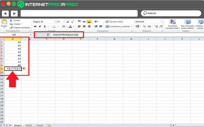
In order to apply this formula you must have a numeric data series either in one column or a row of your spreadsheetin this case we have in the column A between cells A1 and A8, so that the formula is applied as follows: =AVROMDEVP(A2:A8), this will generate the result you see in the image.

Average

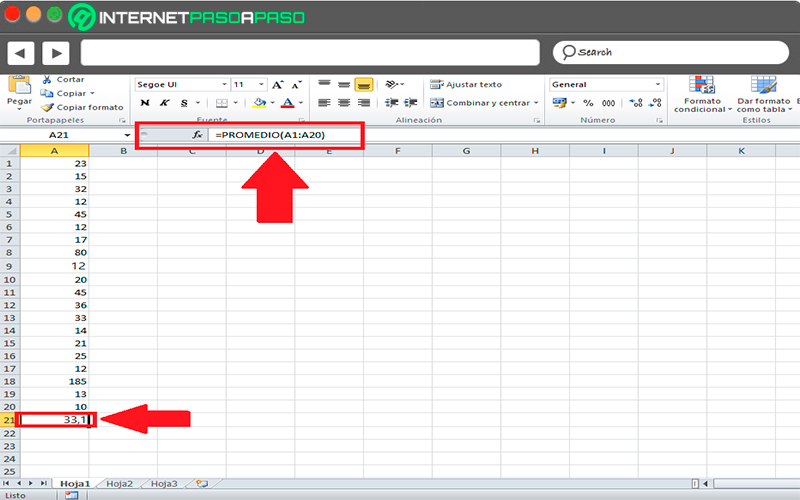
In this case with this function returns the average of the argumentsthat is, if the interval is between cell A1:A20, the formula should be =AVERAGE(A1:A20), this way you will get the average of all the data that is contained between those cells.

AverageA

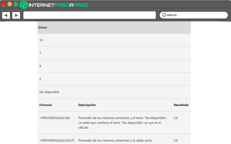
This function takes care of compute the average of the arithmetic mean of the values ​​in the list of arguments. So the formula in this case should be as follows: =AVERAGEA(Value1: Value2). The value 1 is mandatory, while subsequent values ​​are optional. This will depend on the range you want to get the average.

this time arguments can be numbers, references, arrays or names containing numbers, textual representations of numbers, values ​​such as true or false.

For arguments containing true evaluate to 1, while those who contain false are taken as 0. For the arguments of references or arrays that contain text will be taken as 0, and the empty text will also evaluate to 0.

Those arguments that are error values ​​or text they cannot be translate to text so it will throw an error in the result. And in case you don’t want to include logical values, textual representations of numbers as part of the calculation, then it is recommended to use the “Average” function.

Average.yes

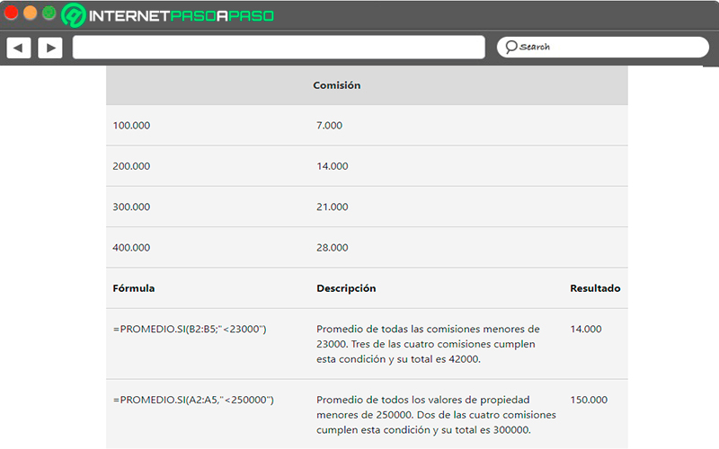
This function takes care of return the average of all cells in a specified range, lwhich ones should meet certain criteria.

The formula in this case is as follows:

• AVERAGEIF(range; criteria; average range).
• Rank is required where one or more cells depending on the average you want to obtain, these can include numbers, names, reference or arrays containing numbers.
• The criteria is also mandatory, The criteria can be number Shape, cell reference or text, expression, among others. In this way it can be said that the criteria can be expressed as 32, “32”, “>32”, “Pears” or B4.
• Average range is optionalthis is the set actual cells whose average will be calculated, if omitted the range will be used.

Regarding the observations, it should be mentioned that in this case they are not taken into account. the range cells that contain true or false values. Now if the range is a blank or text value, the function will return the #DIV0! error value.

In each of the criteria can be used question mark and asterisk wildcard characters. Nor is it necessary that the average range has the same range size and shape.

An example of all this is the following:

count function

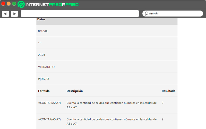
With this function you will have the opportunity to count the number of cells that contain numbers and counts the numbers within the argument list. In this way, it can be used when you need to get the number of entries in a number field of a range or array of numbers.

In this way, we can write the formula for count the numbers in the range A1:A20: =COUNT(A1:A20). The value 1 is required in the formulafirst element for reference the range in which you want count the numbers. While for value 2 is optional, can contain up to 255 elements, cells, or references in which you want to count numbers.

Among the considerations to be taken into account are count arguments that are numbers, dates, text representations of numbers. Also taken into account logical values ​​and textual representations of numbers written directly to the argument list.

Now if the argument is a reference or an arrayit should only consider the numbers of this matrix or reference. Which means that empty cells or logical values ​​are not counted in these cases. To count logical values, text or error values you will need to use the function WILL COUNT.

An example of this COUNT function is as follows:

COUNTA function

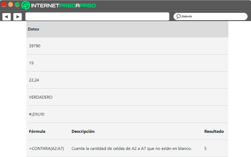
With the COUNTA tool you will have the opportunity to keep track of the number of cells that are not empty in an interval. In this case the formula is written as follows: =COUNTA(value 1: value 2). The value 1 it is required, since it will be the first argument representing the values ​​you want to count. While value 2 is optionalthese additional arguments represent the values ​​that you want to count.

Among the main arguments of this tool is taken into account that the COUNTA function count cells that have any type of information, including the error values ​​and empty text. In the case that you don’t want to count logical values, text or error values, then it is recommended that you use the COUNT function.

An example of all this is the following:

COUNT YES

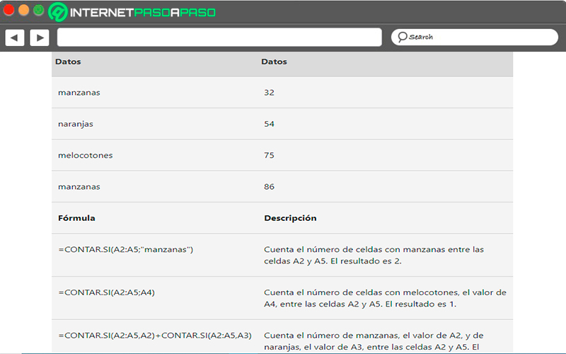
The COUNTIF function is one of the functions of excel statistics most used at the time Count the number of cells that meet a certain criteria. The same can be used for count the number of times a product appears in a certain list.

This function indicates the following: By applying it you will have the opportunity to perform search and what you want to search for. It can be written as follows: =COUNTIF(A2:A5, “plastic”)or also by selecting the cell where the word you want to search for is found =COUNTIF(A2:A5,A4).

So that all this can be much easier to understand, here we leave you the following example:

DIVERT2 function

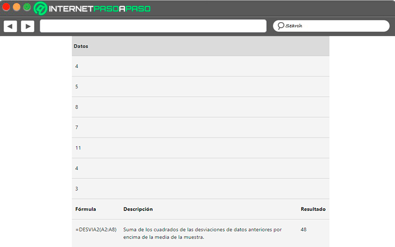
Divert2 is responsible for returning the sum of the squares of the deviations of the data points from the displayed average of the mean.

In this case, the following formula should be used: DEVIATION2(number 1, number 2,…) as in all previous cases number 1 is requiredMeanwhile he number 2.. they are optional. Arguments added to this function include numbers, references, names, or arrays containing numbers. Also taken into account logical values ​​and textual representations of written numbers.

In the case of error values ​​or text cannot be translated since they cause errors in the result.

So that you can understand this a little more here we leave you this example:

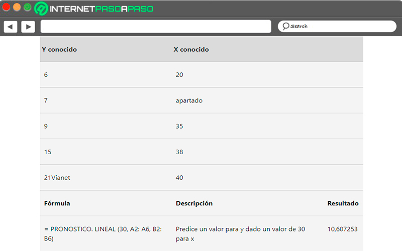
forecast function

In this function you will be able to calculate or anticipate a future value using already existing valuesso a future value is a y value for an x ​​value, existing values are known x-values ​​and y-values. Therefore, the function forecast will be defined with linear regression.

The application of this formula it is done mainly for prDecide future sales of a business, inventory requirements, consumer trendsamong other options.

In the case of this function it is necessary to consider that if the value of X is a non-numeric value, will be thrown the #VALUE or #VALUE!. Yes now the known i known x is empty, or one of the two has more points than the other. In this case it returns the error value #N/A. And lastly, yes the variance of known x is equal to zerothen it is returned the #DIV/0! OR #VALUE!.

For better understanding, here is an example:

Frequency

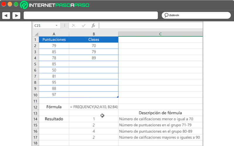
When this formula is applied is done with the aim of calculate the frequency with which they are produced the values within a specific range of data. In this case it returns a vertical array of numbers.

One of the most common reasons for using this frequency function is to count the number of results that fall within a specified range. In this way, the frequency function is specified as a array formula as frequency returns an array.

In order to understand this better, here is an example:

Linear estimate

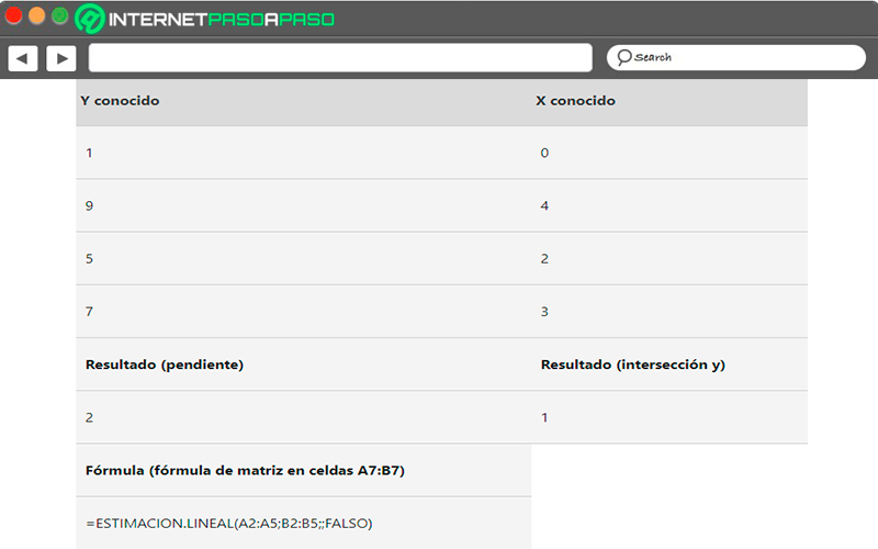
It serves to be able calculate statistics of a line through method of Least Squares, what allows compute the line of best fit to the data. For later return an array that describes the line.

You can also combine what is the estimate.line with other functions in order to compute statistics from other models that are linear in the unknown parameters. Between these Parameters include logarithmic, exponential, power, and polynomial series. This is all because the function returns an array of values ​​that must be specified as array formula.

Regarding the observations that must be taken into account, any straight line can be described with the slope and y-intercept:

• Slope (m): It is used to find the slope of a line, it is always or mostly written as m, it takes two points on the line (X1, Y1) or (X2, Y2), the slope is equal to (Y2-Y1)/(X2-X1).
• Y-intercept (b): is usually defined mostly with the letter (b), y is the value of y at the point where the line intersects on the y-axis.
• The equation of the straight line is y=mx + b. this means that if they know each other the values ​​of m and b can be easily calculated. This allows you to calculate any point on the line inserting the values of Y or X in the equation.

Now if you only know one independent variable X, you can get the slope and intercept values ​​using any of the following formulas:

• Earring: =Index (ESTIMATE.Linear (known_y, known:x), 1)
• Intersection: =ESTIMATE.Linear (known_y, known_x). two)

when it is calculated the estimate.line the accuracy of the calculated line goes to depend on the degree of dispersion of all the data to be evaluated. Yes the data is linear the more accurate the model will be. In this way, linear.estimation makes use of Method of least squares in order to find the best fit for the data.

In order to understand this a little more, here is an example:

MAX function

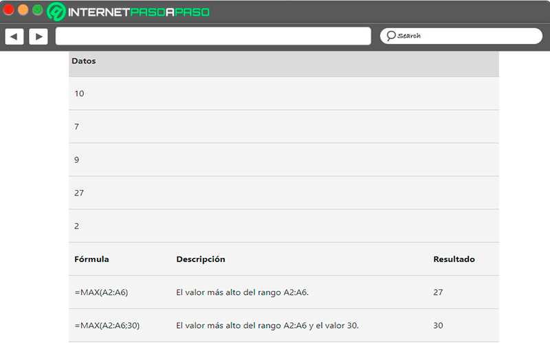
It is frequently used for know the maximum value of a specific set of values. It is mostly used to find out what seller obtained more sales in a month, what was the product that sold the most throughout the year, among many other alternatives.

The arguments of this function can be numbers, names, arrays, or references that have numbers. In addition, it takes into account logical values ​​and textual representations of written numbers. In the event that it is a reference or an array is taken into account just the numbers contained therein.

Now if the argument does not contain numbers, the MAX function will return zero 0. If it’s a text value or error cannot be translated so an error will be generated.

With this in mind, here is an example of such a MAX function:

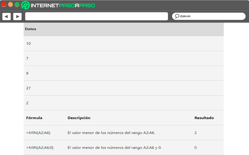
MIN function

In this case, the opposite occurs previous functionis used to find out what is the minimum value of a data set. This means that with it you can know what seller is generating fewer sales, which product takes longer to come out, among many others.

Like the MAX function, arguments can be numbers, arrays, names, and references that contain numbers. Here are taken into account the logical values ​​and the textual representations of numbers written in the argument list.

In the case of arrays and references They will only be taken into account if they have numbers, all empty cells will be taken as zero. The arguments that are text or error values ​​cannot be translatedso they will generate as a result an error.

In order to understand all this better, we leave you the following example:

Earring

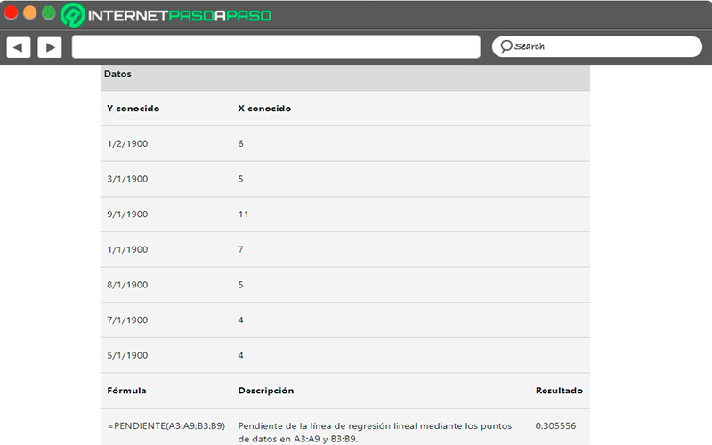
Its purpose is to be able return the slope of a linear regression line which has been created through the data of the known arguments in X and in Y.

So the slope is the vertical distance divided by the horizontal distance between any two points on a line. All of this corresponds to the rate of change in the path of the regression line.

This function has the following arguments:

• Acquaintance_X: is required, and is the set of independent data points.
• Known_Y: is also required and is a cell range or array of dependent numeric data points.

As in most of the functions mentioned above, its arguments must be numbers or references containing numbers. In the case that do not contain these cells will have a value of zero.

If the arguments known_y and known_x it’s found no value or has a different number of data points, the Slope will give the error value #N/A.

So that you can understand this much better, we leave you this example:

It can be said that these are some of the most used functions in the Microsoft Excel program and which will help you to facilitate certain mathematical and statistical operations at the moment of wanting to know certain specific values.

However, there are many other statistical functions available which we present to you in a much more summarized way:

STATISTICAL FUNCTION	DESCRIPTION
CD T.DIST	returns the distribution of Studen’s t.
INV.T.2C	Returns the inverse function of Student’s t-distribution.
INVT.T	This time it returns the value of t of Student’s t-distribution depending on the probability and the degrees of freedom.
Trend	It offers you the values ​​of the linear trend.
Bounded.mean	Throw the inside stocking of a data set.
Quartile.exc	Bring back the quartile of the data set, These are based on the values percentiles from 0 to 1.
HIERARCHY.MEDIA	Returns the hierarchy of a number in a numeric data list.
HIERARCHY.EQV	It also returns the hierarchy of a number in a list of numbers.
COEFFICIENT.R2	Returns the square of the moment coefficient of Pearson product correlation.
MINE	Returns the minimum value in a list of arguments, including numbers, text and logical values.
FASHION.VARIOUS	Came back the vertical array of values that are repeated very frequently in a range of data.
FASHION.ONE	Came back the most common value of a data set.
INV.NORM	Bring back the inverse function of the cumulative normal distribution.
NORM.DIST.N	return what is the cumulative normal distribution.
NEGBINOM.DIST	Bring back the negative binomial distribution.

Common errors when using statistical formulas What are they and how to solve them?

When it’s used the excel program it is more than necessary to have to introduce some formulas to carry out different mathematical operations.

However, on many occasions when they are introduced they end up generating a mistake, so it can be due to many reasons. Whether it’s because entered wrong some sign, a value or any other character corresponding to it.

According to this, here we present the most common mistakes when using statistical formulas:

#WORTH!

It’s one of the most common mistakes when making use of Excel, he himself is provoked when adding text valuesyou enter a text value in a parameter what is a number or when array formulas are used without using the key combination “Control + Shift + Enter” to enter the formula.

if this error is affecting your work in the spreadsheetthe best way to correct it is that only add the numeric values ​​from your data table.

#DIV/O!

This type of error can be generated via different reasonseither because dividing a number by a zero value, divides by an empty cell or when averaging and there are numbers to average.

The best way to solve this is by the mathematical rulesince there is no divide by zero because it will automatically throw you an error.

#NAME?

Another of the most common errors that occur in the functions of Excel Its the #NAME?, it occurs for different reasons, either when uses a function that does not exist in a version of the program or when you make one reference to a defined name that exists in the file.

If this happens to you mistakethen you will need to check that the functions that you are using are available in your version of Excel. The best solution to these problems is have the most recent update of the program on your computer or mobile.

#N/A

If this appears warning then it may be because a value is not found in the VLOOKUP, HLOOKUP, or MATCH functions. It is also generated when operations are performed on a range that has a value N/A. To solve these inconveniences it is better that you look for another name that exists in the table.

#REF!

This error usually occurs when referring to a range that no longer exists. That is, when used in a formula and subsequently deletes a row or column from which the formula refers.

The way to fix this is to avoid delete rows or columns that are reference of some other formula that has been used.

#NUM!

This error usually appears when you end up entering parameters in the functions without respecting the order or when you have a very large number. You have to remember that Microsoft Excel does not allow you to use very large numbers.

This means that the way to correct it is avoiding large numbers or modify and swapping parameters.

#NULL!

If this error has appeared, then you must bear in mind that it is generated when there is an incorrect range in the formula or when there is no intersection between two rangesan example of this would be the following: =SUM(E3 E4), which will end up generating the error.

The most viable solution for this is that use the formulas correctlyespecially at the time of Separate cells with either a colon, comma, or semicolon.

#####

appears when the result that is generated from some formula is too large and cannot be displayed since it does not fit in the cell. The solution for this is expand column width until it appears to you said result.