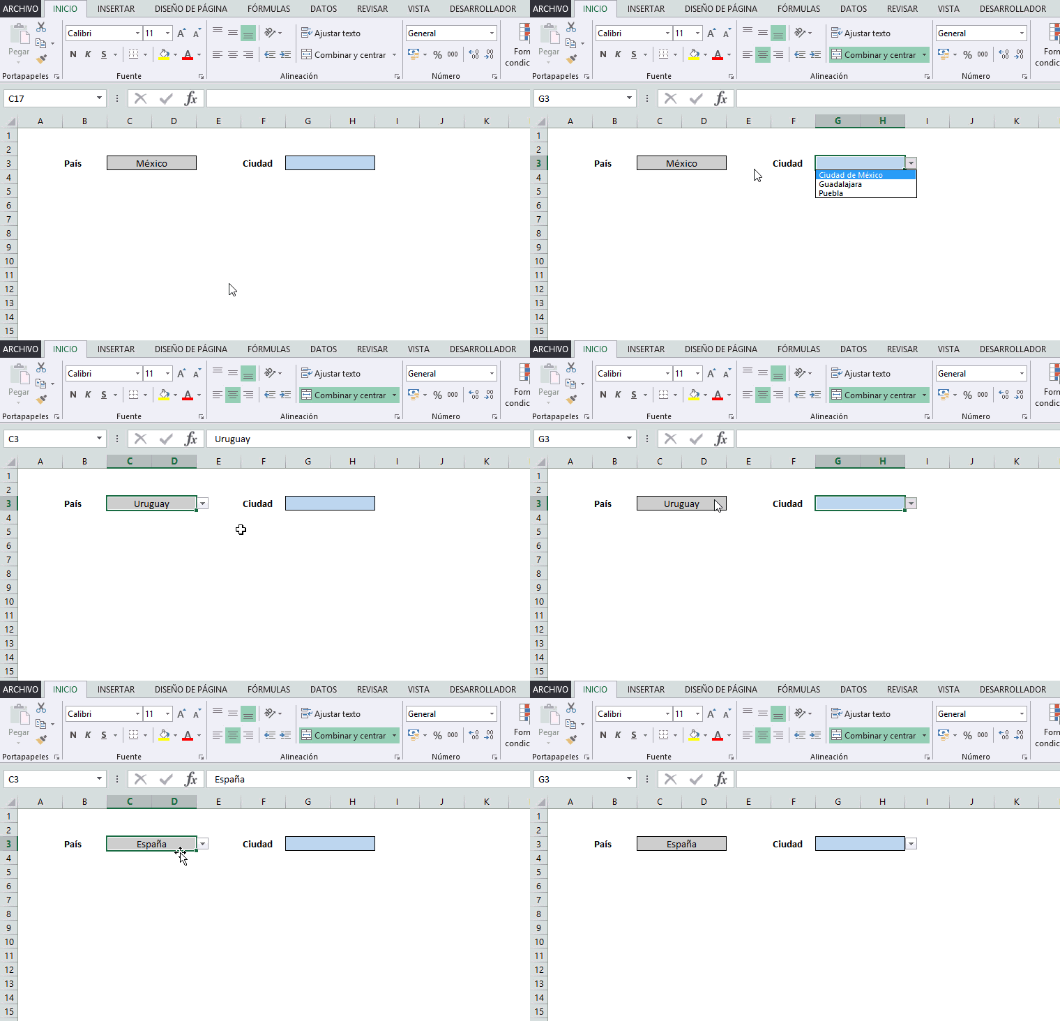
Have we heard of the famous Excel drop-down lists? or do we need to make a drop-down list for our work in Excel and we don’t know how? Here in this guide we will explain all the steps to follow so you can create your list, without any complications.
With these steps you can create the ones you want, wherever and whenever you want, just following them to the letter. If you have an old version of Microsoft Excel, rest assured that we also explain how to do it .
And for those who want to delete the list of one or several cells , we explain in a few clicks how to remove it, allowing the writing of any value inside the cell.
Index:
What is a drop-down list and what is it for in Excel?

A drop-down list is a tool provided by Excel itself. This is an element of the user interface that allows us to select from a list some mutually exclusive options, this is shown as a button that when the cell is selected shows a list.
Many professionals nowadays use this Excel function , since it allows us to make a better organization of information that must be reflected in a sheet.
Also being used for the creation of forms, where they should only be filled in with specific words and with the drop-down list, the person is limited to just writing or marking what is in it. It really has many more utilities , but it all depends on what we are going to do.
Steps to create a drop-down list in a Microsoft Excel cell
The drop-down lists are very useful for our professional development. Here we show you the steps to follow so you can make a drop-down list when and how you want:
- First we must open an Excel sheet , then select the cell we want, so that it becomes a list. If there are several, we only copy the same style in the other cells to repeat.

- Creating a drop-down list is very simple. After having our Excel sheet open, with the box where we will insert our list , we must define those words or options that we want to be in the list. These, we can write next to the picture or in another book.

- At the top of the Excel window we find different tabs, we locate the tab that says “Data” and then we go to the “Data tool ” and click on where it says “ Data validation ”.

- After we click, we will see a small box that has the name “Data validation” . There, under “ Allow ” we display the list you provide and click on the “ List “.

- When we select the option, we are shown other options, including a white field below “Origin”. When we select this, we will have to determine the words we want to be in the drop-down list . These words we had to have determined previously. And finally we give clearlyAccepte.

- With these steps we can make as many drop-down lists as we want. Although we have to remember that to to be able to make this list we must select that cell, where we want the list to be located. If this is not done, the list will be located within the same options, which is not what we are really looking for.

- We can identify that the list is located in the cell when a small arrow is marked down , when we are selecting the cell. If this is not checked we will have to perform all the steps again because the operation was not completed successfully.
How to delete the drop-down list
To remove the drop-down list of a cell we must locate the sheet where we have previously created the list:
- Select the cells in which we want the drop-down list to stop appearing.
- After selecting the cell (s) we go to the tab from “Data”, then to the “Data tool” section and click on “ Data validation “.
- In the small box shown to us, we click on “Any value “, and we finish by clicking on “Accept ” and in this way the drop-down list .
Excel version 2010
Basically, the steps shown above are all we need to know how to create a drop-down list . In the version of the Office 2010 Package (one of the oldest today) nothing changes, nor the positions of the options, which makes it even easier to elaborate our objective. Doing this is more practical, because of difficulty you have nothing. But we must follow the steps to the letter, or else it will not be created.
Tips and Tricks
If what we want is to create a list, but not in cells of the same column or that are non-contiguous cells , we must select the cells by pressing on the keyboard the “Ctrl” key, and when we finish selecting the cells that we want to have the option of drop-down list we stop pressing the key.
Finally, remember that we are placing the “List” option and remove the one that said “Any value ”, meaning that the cells we marked for the list will only allow the deeds of the words on the list. Since when we try to write something else that does not appear inside it, we will get a warning that tells us that we cannot do it.