How to filter and sort information in a Microsoft Excel pivot table? step by step guide

While it is true, Microsoft Excel has been classified as one of the most important office programs throughout history. Which basically consists of an arrangement of rows and columns divided by boxes, so that, like this makes editing and managing spreadsheets easy.

Thus, it is an ideal software for tabulate and organize any type of informationAs for insert numeric data in order to manage them in the best possible way. Taking into account that, it provides numerous tools for order said data and optimize the presentation of the same.

So, one of those tools, consist of Excel pivot tables. Well, they are elements that allow summarize and analyze large amounts of information in a simple way, just by dragging and dropping the different columns that are part of the table. So that, allow you to filter data and here, we will teach you how to do it.

When is it necessary to filter data in an Excel pivot table?

In general terms, pivot tables are useful utilities for summarize a huge stream of data contained in an Excel spreadsheetwith the objective of facilitate their management and analysis, an effective form. For this reason, pivot tables also support the ability to filter information.

In that sense, it is considered that it is necessary to filter data in an Excel pivot table to achieve take large sets of information and from it, create truly detailed in-depth summaries. Whereas, given a remarkable amount of information, sometimes users need greater flexibility and that is why the function of filtering and sorting information has been added.

As a consequence, it is possible insert one or more data segmentations to carry out the filtering in a practical and effective way. Also, there is the possibility to apply filters to any row field of the pivot table through an autofilter which generally works in conjunction with information segmentations in order to distill all the content into a larger instance.

Steps to sort and filter information in an Excel pivot table

Before proceeding to filter or sort the information contained within a pivot table, you need to make the same. To do this, you simply have to choose the entire table in question and go to the program’s options bar, stop there click on the “Insert” tab.

Then in the Tables group, select the option “Pivot table” and choose the location of it (recommended in the same spreadsheet). Having done all of the above, you will have already created your pivot table and from this moment on, you can start filtering and sorting the available data manually or with a data slicer.

First of all, we explain how to do it manually:

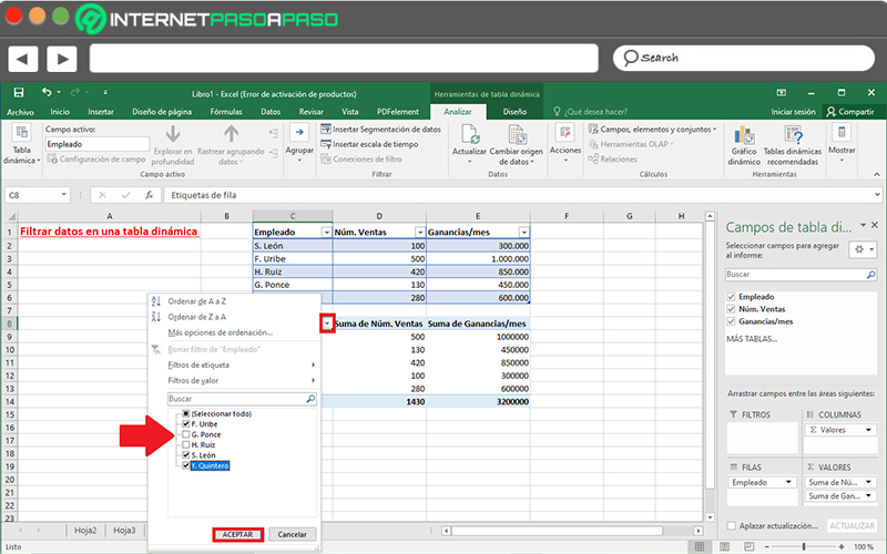
• To filter data manually, just select the down arrow or column header, specifically, on the column you want to filter.
• After that, disable the “Select all” option and click the boxes you prefer to be displayed.
• done that, click the “OK” button and so, all data will be filtered based on the parameters set above.

On the other hand, if you choose to filter data within a pivot table through data segmentationthe steps to follow are different from those just indicated.

Therefore, the following procedure is required to carry it out correctly:

• First of all, you have to select any cell in pivot tableto display the corresponding tools.
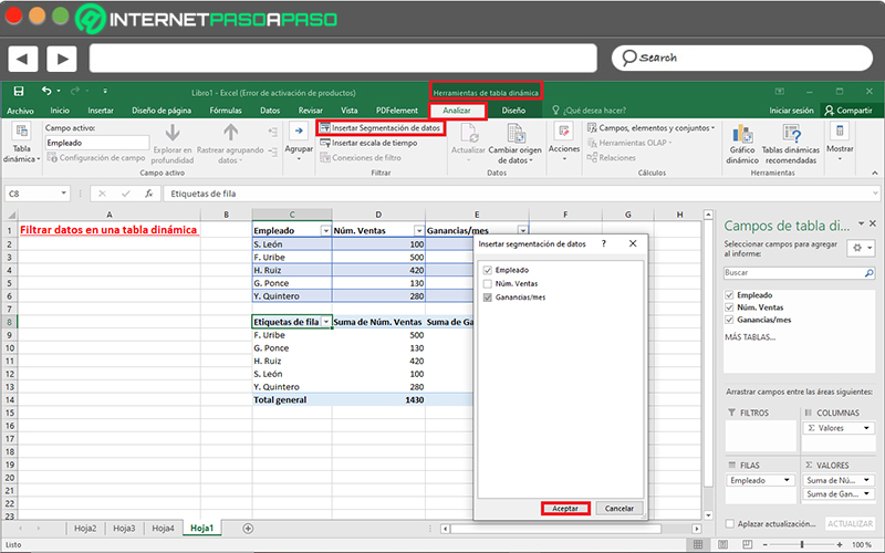
• Then go to the top of Excel and among the options available in “Pivot Table Tools”, click on the tab that says “Analyze”.
• Followed by that, proceed to find the Filter group and then click the option “Insert data segmentation”.
• Now it’s time to choose the fields for which you want to create slicers and when you do, just click the OK button.

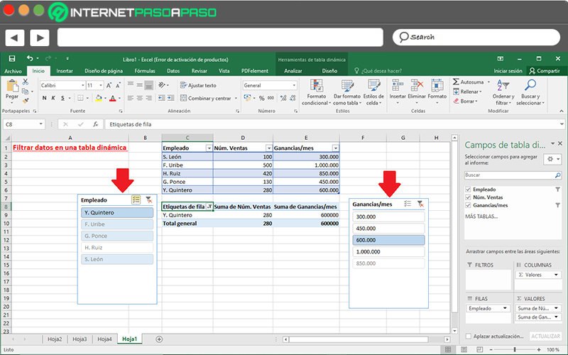
• After the above, the program will take care of presenting a calculation segmentation within the sheet for each selection you made in the previous step. Considering that you can modify its size and place it where you prefer.
• Finally, within the boxes obtained through data segmentation, you can click on the buttons of each filter to choose the elements to display in the original pivot table.