How to use filter larger or smaller values ​​in a Microsoft Excel spreadsheet? step by step guide

Without a doubt this microsoft program It has a large number of tools that will help you achieve a wide variety of solutions for each of your projects on it. This is how it also gives you the possibility of filter larger or smaller data in a spreadsheet.

In this way, filter values ​​in excel has become one of the many interesting options offered the softwaresince this will allow the analysis of a group of data is much simpler and easier to perform. Therefore, with all this you will have the opportunity to get the values that they are within a rangeEither for numbers greater than or less than a certain limit.

In accordance with all this, here we are going to explain a little more about what it is about the function of filtering values ​​in Excel and how you can start using these types of filters in each of your Excel sheetsfor this, follow in detail everything that we will teach you in the post.

Learn how to use the GREATER.OR.EQUAL function in your Excel spreadsheets

Being able to use this function in your Excel sheets is very simple, for this you simply have to follow each of the steps that we are going to indicate below:

• The first thing will be to select the option of “Filter” There you will see different alternatives that you can select, such as the following: “Equals”, “Not equal to”, “Greater than”, “Greater than or equal to”, “Less than”, “Less than or equal to”, “Between”, “Top ten”, “Above average ”, “Below average”.
• Here you must choose any of those options, in that case it will be “greater than or equal to”once selected it will ask you to specify the search criteria.
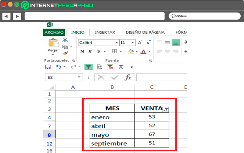
• In this case you have a data table, for what you want it to be perform a search for those values ​​that are greater than or equal to 50.

• Once you enter the data and click on “To accept” the filter order It will only be visible to those values ​​that are greater than or equal to 50. As seen on screen.

If you use the equal to option, then you will have the opportunity to apply a single criterionso only those cells that have that value. This allows you perform precise value lookup for obtain statistical data in a much simpler and faster way.

When you have finished using the data filter, the next thing will be turn it off through the option of “Sort and Filter” in the tab of “Start” located in the menu bar. there you select “Filter” and automatically will remove the date from the header cell.

Steps to get the less than or equal function to work in your Microsoft Excel documents

This software is mainly characterized by automatically evaluating data, where it uses a large number of functions to carry out different types of mathematical operations.

This is the case of the tool “less than or equal to” can be used to indicate a determined criteriato apply it you must establish criteria in advance. In the case that the value of the cell meets the established criteriathen the formula will calculate a “True” value, If the value is greater than the criterion will calculate a “False” value.

To carry out this process, you need to follow the steps that we will indicate below:

• The first thing is to select the cell where the desired result will be displayed and where will insert the function. To do this you must select “Function” and then “Insert” in the top bar menu.
• Now be sure to check the format of the formula in the dialog box to be able to identify the information that has been entered.
• An example of this could be that for the format of the formula YES it is “If(logical_test, value_if_TRUE, value_if_FALSE)”, in this case the logic test It is the main rule for the comparative or conditional criterion. Yes value is TRUEthen a response is generated where the two conditions match and if the value ends turning out FALSEthen a different response is generated if the conditions do not match.
• According to the answers obtained, you should write “=if(“ and then select the cell that contains the value of the criterion or write the value you want. This will look like this: “=if(A3” in the formula bar.
• Now write “(≤)” and then the value you want to contain the criteria to evaluateyou can also choose the cell What do you want to reference?
• All this should be as follows: “if(A3≤100” in the formula bar.
• The next thing is to write “)”, and then press the key “Enter” so that it can be completed function.
• Another way to explore these functions is creating formulas comparison as SUMIF or COUNTIF where you can use the “(≤)”.