Pivot Table Wizard in Microsoft Excel What is it, what is it for and how to use it to facilitate the creation of a pivot table?

Microsoft Excel is the software par excellence when it comes to creating templates, spreadsheets and databases. But often the amount of cells and your information can be overwhelming. Especially for tasks that require a huge flow of data.

This is why the program has a tool called pivot table. which is kind of summary of other content of the same document. It works ideally for process large amounts of data and summarize them according to our needs.

And if that was not enough, Excel also owns a attendee to generate and manage this tool.

What is the Excel pivot table wizard and how does it help us in the preparation of our tables?

As its name indicates, it is a utility that will facilitate the way in which we create our dynamic tables. To do this, it uses pop-up windows that will guide us in all the necessary steps.

It does it through simple questions that allow us to understand the function of each stage of elaborationthe utility will guide us until the pivot table is ready to be configured.

What are the benefits of using Excel’s PivotTable Wizard?

It should be noted that it is very easy to use. And taking into account the level of knowledge that is required when handling a pivot table, the assistant works in a very didactic way. For this reason it is recommended for people who are just entering the world of Excel tables.

However, it is worth mentioning which also has some drawbacks relative. One of them is that since version 2007 of the software, the wizard does not appear inside the ribbon and activating it results in a series of extra steps when creating a table.

In this sense, a second characteristic is that the same result can be reached without using the wizard. In this way we will save several steps, although it is not recommended for the first few times. Since the utility can be very instructive.

The way to create a pivot table without the wizard is through the menu “Insert”. In the section “Boards”it’s found “Dynamic table”.

Learn how to use Excel’s pivot table wizard step by step to create a

As we mentioned before, the quick access for this tool not found in the ribbon from versions 2007 onwards.

However, it is possible to add it by performing these steps:

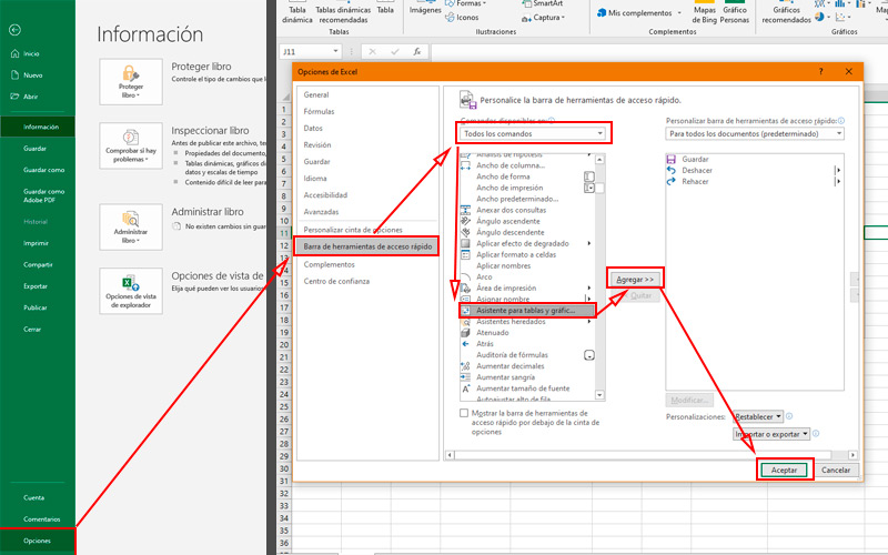
• Inside of the excel document you are working go to the tab “File, Archive”located on the ribbon.
• Inside it you will find the button. “Options” at the bottom of the screen.
• Clicking on it will open the vwindow of this category.
• In the Side panelclick on “Quick-access tool bar”.
• You’ll see two sectors defined. On the one hand, available commands to add to the toolbar and on the other those who are already in it.
• In the left columnchange “Most used commands” by “all commands”.
• In it, search and select “PivotTable and PivotChart Wizard”. (Note that they are in alphabetical order)
• Press the button “Add”.
• And finally “To accept”.

Once these steps have been completed, you will find the wizard in the upper left corner of the program. And now that you have this button, all that remains is start putting it into practice. For this you will have to apply the wizard on a previous table. This must be ordered and with the same types of values ​​for each column or row.

Then follow these steps:

• Press the button we just created. Or if you prefer, you can access it through a keyboard shortcut. “Alt+T+B” if Excel is in Spanish or “Alt+D+P” if it is in English.
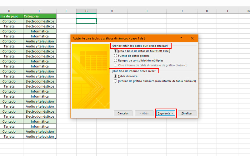
• will appear a small window. in which you must indicate where the data you will use is located for the pivot table. In the example we will use one that is in the same document.
• You must also select the analysis type that you will create, choosing between a pivot table or a graphic.
• Having decided this, we press “Following”.

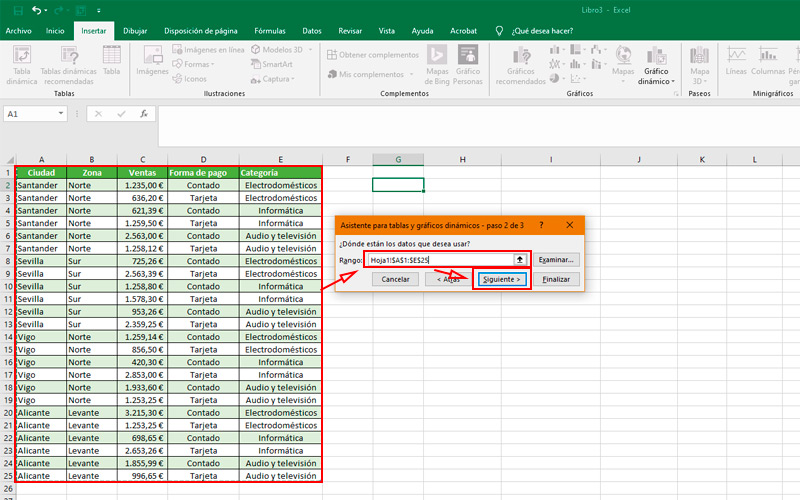
• In the next box you must indicate the cells contain the data you want to use. To do this you just have to drag the cursor over them while keeping the main button pressed.
• Press “Following”.

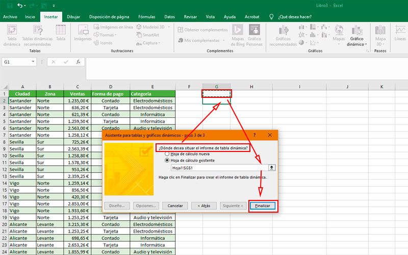
• In the last window of the wizard you have to indicate Where on the sheet will the pivot table be placed?. It is simply a matter of selecting the cell that will serve as the upper left corner of it.
• To finish, press “To finalize”.

Once these steps are completed, a box will be displayed in which the pivot table will be located and an annex to the right of the screen where you will need to configure it.