How to use the information search functions of Microsoft Excel? step by step guide

Within Excelyou can find Functions of searching and referencing. With them, you can locate within spreadsheet different values ​​according to the criteria you specify in your search.

In this sense, it is a great tool for return cell reference information. Each of these functions has a specific syntax and you can take advantage of them depending on your needs.

Here we will talk about how to use excel’s information search functions with a detailed step-by-step guide.

What are lookup functions and what are they for in my Excel spreadsheets?

With the help of excel search functionsthe user has the possibility to find within a spreadsheet any type of information that it requires. To make use of these functions, simply write the formula corresponding to each case.

In this way, there is different search and reference functions that can make your work easier Excel.

These are:

• ADDRESS: help to return a reference as text within a single cell of a spreadsheet.
• AREAS: sample the number of areas of a reference.
• TO CHOOSE: offers the possibility of choose a value from a list of values.
• COLUMN: shows the column number of a reference.
• COLUMNS: shows the number of columns in a reference.
• FILTER: available in Office 365 and allows filter a range of databased on criteria defined by the user.
• FORM EXT: for Office 2013 versions. Shows the formula in the given reference as text.
• IMPORT DYNAMIC DATA: available in the Office 2010 version. Show data stored in a pivot table report.
• SEARCHH: It allows search the top row of an array and returns the value of the specified cell.
• HYPERLINK: help to create a shortcut or jump which opens a document stored within a network server, on the Internet, etc.
• INDEX: choose a value of a reference or an array.
• INDIRECT: sample a reference indicated by a text value.
• SEARCH: allows to get values ​​of a vector or matrix.
• COINCIDE: find values ​​of a reference or matrix.
• OFFSET: sample a reference offset about a specified reference.
• ROW: sample the row number of a reference.
• ROWS: sample the number of rows in a reference.
• RDTR: It allows retrieve data in real time from a program compatible with automation COM.
• ORGANIZE: available in Office 365 and sort the contents of a range or an array.
• SORT BY: available in Office 365. Sort the contents of a range or array according to the values ​​of a corresponding range or matrix.
• TRANSPOSE: shows the transpose of a matrix.
• UNIQUE: available in Office 365. Returns a list of unique values ​​from a range or list.
• CONSULTAV: It allows search the first column of an array and moves on horizontal down the row, with the goal of returning the value of a cell.
• SEARCHX: available in Office 365. Allows the user to search a range or array and return an element corresponding to the first match it finds. It should be mentioned that in case of no match, XLOOKUP helps to return the closest match (approximate).
• XMATCH: available in Office 365. Shows the relative position of an element in an array or range of cells.

Steps to use the information search functions in Excel correctly

take advantage of the information search functions within ExcelIt is easier than it seems to be.

Therefore, we will explain step by step how to do it correctly in each case:

SEARCH function

The use of this function is recommended to users when they need search within a single row or column and find a value from the same position in a second row or column.

Specifically LOOKUP has two options to use, vector form and matrix form:

SEARCH in vector form

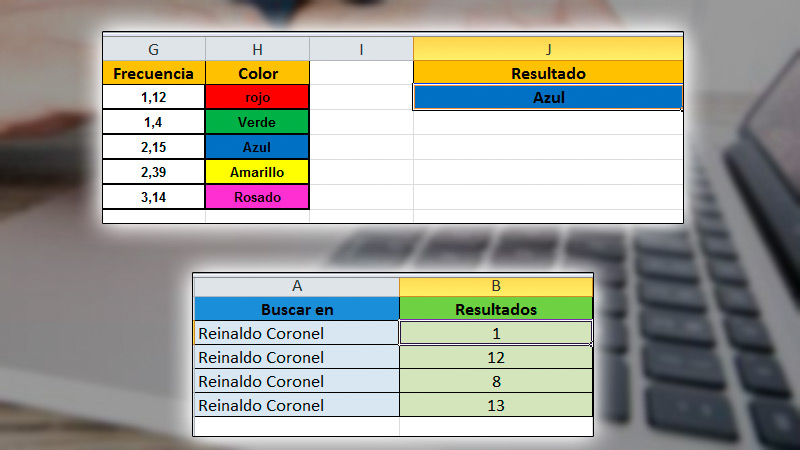
With the vector shapeyou may search a range of a row or column (referred to as a vector) a certain value. In this way, returns it from the same position but in a second rank.

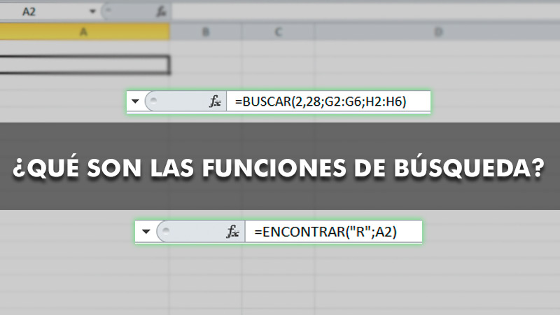
The corresponding syntax is: LOOKUP(lookup_value, comparison_vector, [vector_resultado]).

In addition, it has the following arguments:

• Lookup_value (Required): this is the value you look for with the LOOKUP function within the first vector. This can be a text, number, logical value, and even a reference name indicating a specific value.
• Comparison_Vector (Required): refers to a range that contains only one row or column. These can be texts, numbers or logical values.
• Result_vector (Optional): is a range containing only one column or row. It needs to be the same size as the lookup_vector.

Finally, so that these formulas show the resultsit may be necessary select them in the spreadsheet. To do this, press F2 and then Enter. Apart from that, you can adjust column widths to see all the data, in case you require it.

SEARCH in matrix form

With the array form of LOOKUPIt can find the specified value in the first column or row of an array. With it, the value of the same position in the last row or column of the matrix is ​​displayed.

Its use is recommended in case the values ​​you are looking for are located in the first row or column of an array.

The syntax for this is: LOOKUP(lookup_value, array).

Other than that, It has the following arguments:

• Lookup_value (Required): is the value that the LOOKUP function looks for. It can be a text, number, reference name of a value, and even a logical value. In addition to that, you should know that if you can’t find the lookup_value, use the largest value in the array that is less than or equal to the lookup_value. Also, if said value is less than the first row or column (according to the dimensions of the array), a #N/A error value will be returned.
• Matrix (Required): corresponds to the range of cells containing numbers, text, or logical values ​​that you want to compare lookup_value to.

Function FIND and FINDB

With these functions, the user can search for a text string within a second string. In this way, returns the number of the starting position of the first string from the first character of the second.

Specifically FIND has two options to use, FIND and FINDB:

FIND function

Always count each character as 1no matter if it is from single byte or double byteregardless of the default language setting.

The syntax used in these cases is: (search_text, inside_text, [núm_inicial]).

FINDB function

takes care of count each double-byte character as 2if enabled language editing option that admits DBCS. After that, set as default language. If not, the function will count each character as 1.

The syntax for FINDRB is: (search_text, inside_text, [núm_inicial]).

In both cases, the arguments of these functions are:

• Search_text (Required): text you want find.
• Inside_text (Required): text containing the text you want find.
• Start_num (Optional): helps specify the character from which to start the search.

Remarks What to keep in mind when using these Excel functions?

All functions that you can perform within ExcelThey have a series of very helpful tips that will allow you to work with them more easily and avoid errors during your jobs.

Some observations to consider with the SEARCH function are:

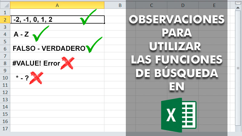
• if you can’t find the lookup_value with the SEARCH function, you should know that the function returns the largest value in comparison_vectorwhich is less than or equal to lookup_value.
• In case the lookup_value is better than the smallest value of the comparison_vectorSEARCH will return a #N/A error value.

On the other hand, the observations corresponding to FIND and FINDRB are:

• Both are case sensitive. Besides, do not allow the use of wildcards. For that reason, if you don’t want to perform such a distinguished search, use SEARCH and SEARCHB.
• search_text must not contain wildcards.
• In case search_text is “” (empty text)the FIND function will match the first character of the search string. This means the start_num character or 1.
• If search_text is not in within_textFIND and FINDB will throw the error #VALUE! or #VALUE!.
• If start_num is not greater than zero, the error #VALUE! error #VALUE!.
• If start_num is greater than the length of inside_textthe error message will also be displayed #VALUE! error #VALUE!.
• Use start_num to skip a specific number of characters.